library(tidyverse)
library(broom)

df <- read_csv("https://raw.githubusercontent.com/yesols/aou-workshop/refs/heads/main/data/final_dataset2.csv")
head(df)Statistical Analysis and JupyterLab Tips
1 Learning Objectives
In this last session, we will perform statistical tests and fit models that are common in medical research. Detailed discussions on statistics are beyond the scope of this workshop. If you want to learn more about these tests, check out links provided in Additional Resources.
At the end of Session 4, learners will be able to:
- Perform t-test, ANOVA, chi-square tests in R.
- Fit regression models: simple linear regression, multiple linear regression, logistic regression
- Obtain odds ratios from logistic regression models.
- Familiarize with navigating JupyterLab
2 Setup
We will load packages and read in the data file. In addition to tidyverse, we will also import broom package which has convenient functions to make results output very readable.
# A tibble: 6 × 14
  person_id year_of_birth race    sex_at_birth condition_concept_id
      <dbl>         <dbl> <chr>   <chr>                       <dbl>
1         1          1987 Unknown Male                           NA
2         2          1987 Asian   Female                         NA
3         3          2004 Asian   Male                           NA
4         4          1944 Black   Male                           NA
5         5          1941 Asian   Male                           NA
6         6          2006 Other   Male                           NA
# ℹ 9 more variables: condition_start_date <date>,
#   condition_source_value <chr>, drug_concept_id <dbl>,
#   drug_exposure_start_date <date>, true_exposure_status <chr>, SBP <dbl>,
#   age <dbl>, condition_status <dbl>, exposure_status <dbl>
3 Two-Sample T-Test
We use t-test for continuous vs binary variables. Let’s test if there is a statistically significant difference in mean Systolic Blood Pressure (SBP) between participants with and without the condition (condition_status).
By default, R executes a Welch two-sample t-test, which does not assume equal variances between groups. This is generally the preferred approach for clinical data.
t_result <- t.test(SBP ~ condition_status, data = df)
print(t_result)
    Welch Two Sample t-test

data:  SBP by condition_status
t = 0.20451, df = 74.577, p-value = 0.8385
alternative hypothesis: true difference in means between group 0 and group 1 is not equal to 0
95 percent confidence interval:
 -4.953265  6.086527
sample estimates:
mean in group 0 mean in group 1
       117.3881        116.8214
4 One-Way ANOVA
For testing continuous variables in more than 2 categories in a variable, we use one-way ANOVA. Let’s test if there is a statistical difference in mean SBP among sex groups (male, female, other)
# Execute One-Way ANOVA
anova_model <- aov(SBP ~ sex_at_birth, data = df)

# Output the ANOVA table (Degrees of freedom, Sum of Squares, F-value, p-value)
summary(anova_model)
Df Sum Sq Mean Sq F value Pr(>F)
sex_at_birth 2 174 87.08 0.416 0.661
Residuals 92 19258 209.33
5 observations deleted due to missingness5 Pearson’s Chi-Square Test
If you want to test associations between categorical variables, use Pearson’s Chi-square test. In our example, we will see if drug exposure (exposure_status) is associated with MCI/dementia (condition_status).
To execute a Chi-squared test, you must pass a contingency table into the chisq.test() function.
# Generate the base R contingency table and pass it to the test
chi_sq_result <- chisq.test(table(df$condition_status, df$exposure_status))
print(chi_sq_result)
    Pearson's Chi-squared test with Yates' continuity correction

data:  table(df$condition_status, df$exposure_status)
X-squared = 20.931, df = 1, p-value = 4.76e-06
Note
If any expected cell count is less than 5, R will generate a warning. In such cases, fisher.test() should be used instead.
6 Simple Linear Regression
To see the relationship a continuous dependent variable and a continuous independent variable, we can use simple linear regression. We will fit a linear regression model for SBP and age. We use lm() function for fitting linear regression models.
# Fit the linear model
lm_model <- lm(SBP ~ age, data = df)

# Base R summary (verbose)
summary(lm_model)
Call:
lm(formula = SBP ~ age, data = df)

Residuals:
     Min       1Q   Median       3Q      Max
-30.1453  -6.0564   0.9969   5.9673  22.3843

Coefficients:
            Estimate Std. Error t value Pr(>|t|)
(Intercept) 90.34318    2.92574  30.879  < 2e-16 ***
age          0.50592    0.05148   9.827 4.75e-16 ***
---
Signif. codes:  0 '***' 0.001 '**' 0.01 '*' 0.05 '.' 0.1 ' ' 1

Residual standard error: 10.12 on 93 degrees of freedom
  (5 observations deleted due to missingness)
Multiple R-squared:  0.5094,    Adjusted R-squared:  0.5041
F-statistic: 96.57 on 1 and 93 DF,  p-value: 4.754e-16
You can use tidy() function from broom package to display the model neatly as a dataframe:
library(broom)
tidy(lm_model)
# A tibble: 2 × 5
term estimate std.error statistic p.value
<chr> <dbl> <dbl> <dbl> <dbl>
1 (Intercept) 90.3 2.93 30.9 1.13e-50
2 age 0.506 0.0515 9.83 4.75e-16We learned how to create scatter plots in the last session. We can overlay regression fit to the scatter plot easily with ggplot2, using geom_smooth().
ggplot(df, aes(x = age, y = SBP)) +
  geom_point(alpha = 0.5, color = "darkblue") +
  geom_smooth(
    method = "lm",
    color = "red",
    fill = "lightcoral",
    alpha = 0.3
  ) +
  labs(
    title = "Linear Regression: Systolic Blood Pressure by Age",
    x = "Age (Years)",
    y = "Systolic Blood Pressure (mmHg)"
  ) +
  theme_minimal()
`geom_smooth()` using formula = 'y ~ x'Warning: Removed 5 rows containing non-finite outside the scale range
(`stat_smooth()`).Warning: Removed 5 rows containing missing values or values outside the scale range
(`geom_point()`).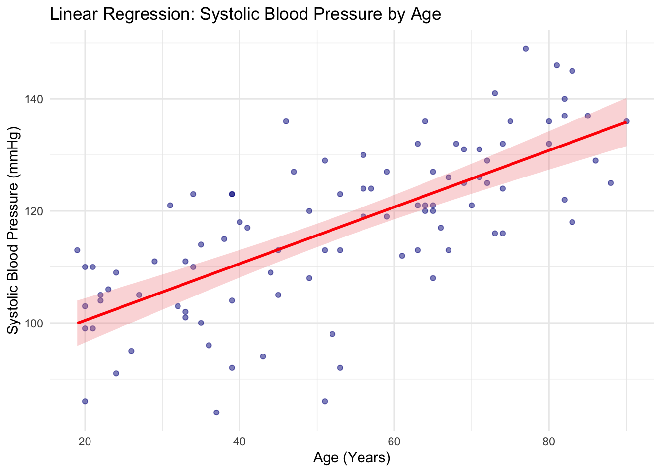
7 Multiple Linear Regression
We use multiple linear regression to see the relationship between one continuous dependent variable and two or more independent variables. In medical research, multiple linear regression is often used as a way to adjust for confounding variables.
We will fit a model to describe the relationship between SBP and age again, but will add sex. To include more independent variables, we simply add variable names to the formula using +:
lm_adj_model <- lm(SBP ~ age + sex_at_birth, data = df)
summary(lm_adj_model)
Call:
lm(formula = SBP ~ age + sex_at_birth, data = df)

Residuals:
     Min       1Q   Median       3Q      Max
-29.3473  -5.4471   0.5786   6.7308  21.8585

Coefficients:
                  Estimate Std. Error t value Pr(>|t|)
(Intercept)       89.63749    3.13686  28.576  < 2e-16 ***
age                0.50411    0.05207   9.681 1.19e-15 ***
sex_at_birthMale   1.31476    2.19149   0.600    0.550
sex_at_birthOther  1.86637    4.18336   0.446    0.657
---
Signif. codes:  0 '***' 0.001 '**' 0.01 '*' 0.05 '.' 0.1 ' ' 1

Residual standard error: 10.21 on 91 degrees of freedom
  (5 observations deleted due to missingness)
Multiple R-squared:  0.5118,    Adjusted R-squared:  0.4957
F-statistic:  31.8 on 3 and 91 DF,  p-value: 3.764e-14
Using broom:
tidy(lm_adj_model)# A tibble: 4 × 5
term estimate std.error statistic p.value
<chr> <dbl> <dbl> <dbl> <dbl>
1 (Intercept) 89.6 3.14 28.6 3.14e-47
2 age 0.504 0.0521 9.68 1.19e-15
3 sex_at_birthMale 1.31 2.19 0.600 5.50e- 1
4 sex_at_birthOther 1.87 4.18 0.446 6.57e- 18 Logistic Regression
Because logistic regression is not discussed in your Research Methods course, I will provide a little bit of background before we learn the R command.
8.1 Theoretical Background
Standard linear regression predicts a continuous outcome \(Y\) based on a linear combination of predictors \(X\): \[Y=\beta_0+\beta_1X_1+\dots+\beta_pX_p\]
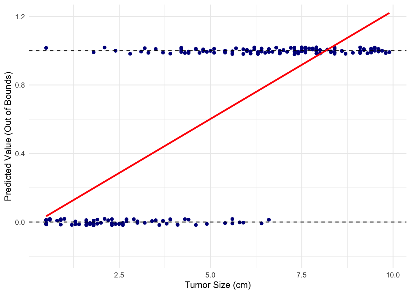
When applied to a binary clinical outcome (absence or presence of a disease, benign or malignant. alive or dead), the linear fit does not make sense when trying to model binary outcomes.
Suppose we have a dataset of tumor sizes from 200 patients and whether they are benign (0) or malignant (1). A linear regression model (red line) would look like this:
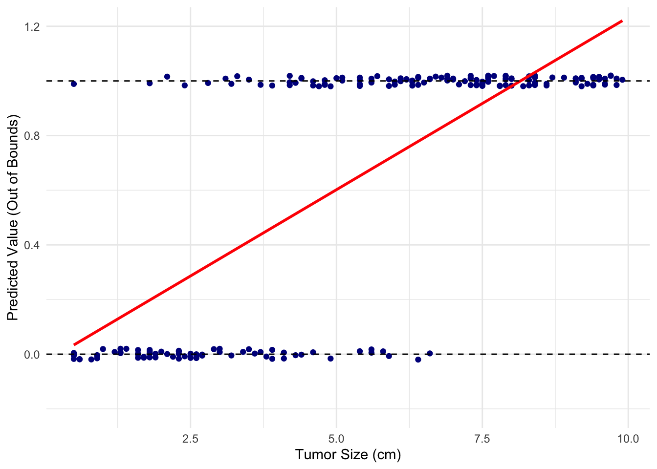
It does not seem like a good fit at all!
For this kind of scenarios, we use logistic regression. In a logistic regression model, the outcome \(Y\) is “logit”-transformed, i.e., turned into log-odds. \[\ln\left(\frac{p}{1-p}\right)=\beta_0+\beta_1X_1+\dots+\beta_pX_p\] Solving this equation for \(p\), the probability of a given outcome (tumor is malignant): \[p=\frac{1}{1+e^{-(\beta_0+\beta_1X_1+\dots+\beta_pX_p)}}\]
Now we have a valid probability that enables us to predict malignancy based on the tumor size.
The fact that logistic regression models the log-odds of a binary outcome provides a useful mathematical property: the coefficients, \(\beta_1, \beta_2, \dots\), of the independent variables, \(X_1, X_2, \dots\), represent the log of the odds ratio for a one-unit increase in those variables. If the independent variables are binary (e.g., \(1\) for exposed and \(0\) for unexposed), the coefficient specifically represents the log odds ratio of the outcome for the exposed group compared to the unexposed group. That means the exponent of a coefficient, i.e., \(e^{\beta_1}\), etc, represent odds ratio of the corresponding variable.
So, logistic regression is primarily utilized for two purposes: predictive modeling and effect estimation. In predictive modeling, it is used to calculate the probability of a binary outcome. In inferential statistics, it is used to calculate adjusted odds ratios to measure the association between exposures and outcomes. This makes it the standard modeling approach for retrospective case-control studies, where calculating relative risk is mathematically invalid.
8.2 Application
We will fit a logistic model on our practice dataset now, to see if there is any association between drug exposure and dementia outcome, while adjusting for age and sex. We use glm() function for this purpose. The argument, family = "binomial", specifies that we want logit link (i.e., \(\ln\left(\frac{p}{1-p}\right)\)), which is what makes it logistic regression as opposed to other types.
# Fit the multivariable logistic regression model
logistic_model <- glm(
  condition_status ~ exposure_status + age + sex_at_birth,
  data = df,
  family = "binomial"
)
summary(logistic_model)
Call:
glm(formula = condition_status ~ exposure_status + age + sex_at_birth,
    family = "binomial", data = df)

Coefficients:
                  Estimate Std. Error z value Pr(>|z|)
(Intercept)       -2.18139    0.83531  -2.611  0.00902 **
exposure_status    2.15673    0.50529   4.268 1.97e-05 ***
age                0.01018    0.01301   0.783  0.43383
sex_at_birthMale  -0.39916    0.52993  -0.753  0.45131
sex_at_birthOther  0.22907    0.90841   0.252  0.80091
---
Signif. codes:  0 '***' 0.001 '**' 0.01 '*' 0.05 '.' 0.1 ' ' 1

(Dispersion parameter for binomial family taken to be 1)

    Null deviance: 122.173  on 99  degrees of freedom
Residual deviance:  98.024  on 95  degrees of freedom
AIC: 108.02

Number of Fisher Scoring iterations: 4
You can obtain the odds ratio by expoentiating the coefficients manually, using exp() function, or the tidy() function from broom package can do this for you as well as confidence intervals.
# Extract exponentiated coefficients (adjusted Odds Ratios) and CIs
library(broom)
tidy_results <- tidy(
  logistic_model,
  exponentiate = TRUE,
  conf.int = TRUE
)
print(tidy_results)
# A tibble: 5 × 7
term estimate std.error statistic p.value conf.low conf.high
<chr> <dbl> <dbl> <dbl> <dbl> <dbl> <dbl>
1 (Intercept) 0.113 0.835 -2.61 0.00902 0.0191 0.525
2 exposure_status 8.64 0.505 4.27 0.0000197 3.31 24.3
3 age 1.01 0.0130 0.783 0.434 0.985 1.04
4 sex_at_birthMale 0.671 0.530 -0.753 0.451 0.235 1.91
5 sex_at_birthOther 1.26 0.908 0.252 0.801 0.193 7.35
ImportantModel Diagnostics
Regression methods such as linear regression and logistic regression rely on statistical assumptions about underlying data. Before making an inference based on a modeling result, it is critical to check these assumptoms through model diagnostics. Refer to your statistics text or Additional Resources link on the left sidebar to learn more.
10 Documenting with Markdown Cells
Markdown is a lightweight markup language that is easy to use for simple text formatting. In Jupyter Notebooks, markdown is often used for sectioning the documents and annotating the code. You can change a cell from “Code” to “Markdown”, type in the section headings or your comments, and running the cell will render the markdown formatting.
Here are a few common markdown examples:
# Main Heading
## Subheading
### Smaller Heading

**Bold Text**
*Italic Text*

- Bullet point 1
- Bullet point 2
  - Indented bullet point

1. Numbered list
2. Numbered list
And here is what that exact formatting looks like once the cell is executed:
11 Pivoting Survey Data (Long to Wide)
If you pull multiple survey items, the query result will be in a “long” format, where each row corresponds to a single survey item per person. This means that there will be multiple rows per person. We typically want a dataframe where each row is a unique participant and questions are columns with answers as values. We can reshape the dataframe from a long format to a wide format using pivot_wider() function.
First, let’s look at a mock example of what your raw survey data might look like:
# Create a mock "long" survey dataframe
survey_long <- data.frame(
  person_id = c(1, 1, 1, 2, 2, 2),
  question = c("1535717", "1585723", "1585729", "1535717", "1585723", "1585729"),
  T_DISP_answer = c("Yes", "Never", "Good", "No", "Always", "Fair")
)

head(survey_long)
person_id question T_DISP_answer
1 1 1535717 Yes
2 1 1585723 Never
3 1 1585729 Good
4 2 1535717 No
5 2 1585723 Always
6 2 1585729 FairNow, we will pivot this dataframe so the question IDs become our new column names, and the T_DISP_answers become the values inside those columns.
# Reshape to wide format
survey_wide <- survey_long %>%
  pivot_wider(
    id_cols = person_id,               # The column that identifies unique rows
    names_from = question,             # The column containing your new column names
    values_from = T_DISP_answer,       # The column containing the actual answers
  )

head(survey_wide)
# A tibble: 2 × 4
person_id `1535717` `1585723` `1585729`
<dbl> <chr> <chr> <chr>
1 1 Yes Never Good
2 2 No Always Fair 12 Other Tips
Tab completion: Use tab key to see suggested functions or to drill down a file path.
Datetime: In All of Us data, you will often see a datetime column with values in a format, “YYYY-MM-DD 00:00:00 UTC”. When you read in a CSV file, this type may be read as character data type. In that case, use as_date() function from lubridate package (included when you load tidyverse).
R objects vs. files: When you run commands like df <- read_csv("my_data.csv"), you are reading a copy of the file contents into the Jupyter environment as an R object (the dataframe df). This object exists solely in memory (RAM), not in any directories unlike files. To list all those objects that are currently in your environment, use ls() function. Also note that if your notebook kernel restarts or your session times out, all R objects are erased from memory and must be reloaded by re-running your code.
%in% operator: %in% checks whether an element exists in a vector. This can be useful when you want to filter rows with certain values. For example: person_df %>% filter(sex_at_birth %in% c("Male", "Female"))
Where am I?: Use getwd() function to check the current directory you’re in. This may become relevant when you’re constructing a relative path of a file.